Graphs: What Production Systems Teach Us

A recommendation system worked flawlessly in testing: sub-100ms response times, accurate suggestions, clean architecture. Two weeks after launch, response times ballooned to 8+ seconds, memory usage spiked to 94%, and the team was scrambling to roll back.

The problem wasn't the algorithm, it was the graph data structure. They'd implemented their graph as nested dictionaries because it felt natural in Python and worked well with their 50,000-node test dataset. In production, with 12 million users and 300 million edges, every traversal meant dictionary lookups nested four levels deep. The garbage collector thrashed constantly.

The fix: replacing nested dictionaries with a compressed adjacency structure using integer indices instead of object references. Memory dropped from 94% to 31%. Response times returned to 90ms.

What are graphs?

Graphs are data structures consisting of nodes (vertices) and edges (connections between nodes). Put plainly, graphs are the natural structure when relationships between entities matter as much as the entities themselves.

# PROBLEMATIC: Nested dictionaries with object references
# Memory: 94% usage on 12M users, 300M edges
graph_bad = {
    'user_1': {
        'friends': {'user_2': {'since': '2021-03-15', 'strength': 0.8}},
        'follows': {'user_3': {'since': '2022-01-20'}},
    },
    # Each nested dict carries vtable pointers, padding, metadata
}
 
# FIXED: Compressed adjacency with integer indices
# Memory: 31% usage on same dataset
class CompressedGraph:
    def __init__(self):
        self.node_to_id = {}      # 'user_1' -> 0
        self.id_to_node = []      # 0 -> 'user_1'
        self.edges = []           # [(source_id, target_id, edge_type_id)]
        self.edge_types = {}      # 'friends' -> 0 (interned strings)
        self.offsets = []         # Index into edges for each node
    
    def add_node(self, node):
        if node not in self.node_to_id:
            self.node_to_id[node] = len(self.id_to_node)
            self.id_to_node.append(node)
        return self.node_to_id[node]
    
    def neighbors(self, node_id):
        start = self.offsets[node_id]
        end = self.offsets[node_id + 1] if node_id + 1 < len(self.offsets) else len(self.edges)
        return self.edges[start:end]  # Contiguous memory access

What are the different types of graphs? 

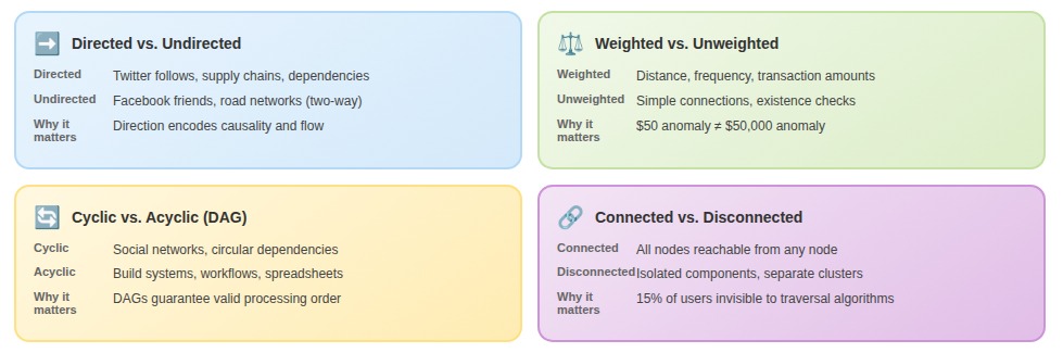
• Directed vs. undirected: Twitter's follower graph is directed: I can follow you without reciprocation. Facebook's friend graph is undirected: friendship is mutual by definition. One supply chain team modeled supplier relationships as undirected. Three months in, they couldn't answer: "If this supplier fails, which downstream products are affected?" Direction encodes causality. They'd thrown it away.
• Weighted vs. unweighted: Weights carry domain-specific meaning: distance in road networks, interaction frequency in social graphs, transaction amounts in fraud detection. A fraud team spent weeks building an unweighted transaction graph before realizing they needed dollar amounts to distinguish a $50 anomaly from a $50,000 one.
• Cyclic vs. acyclic: Cycles mean you can follow edges back to where you started. This sounds theoretical until you're debugging an infinite loop in a dependency resolver. DAGs (directed acyclic graphs) guarantee a valid processing order; that's why they're everywhere in build systems, workflow orchestration, and spreadsheet recalculation.
• Connected vs. disconnected: Disconnected graphs have isolated components. One recommendation system failed silently for 15% of users because they were in a disconnected component, invisible to traversal algorithms.

Each property is a constraint that enables certain operations and prevents certain bugs. Choose wrong, and you'll rebuild.

Why textbook graph implementations fail in production

Textbook implementations treat memory as infinite. A knowledge graph for document analysis followed classic patterns: each node was a full object with properties stored inline, edges were bidirectional pointers with relationship metadata. Memory usage ran 40x higher than raw data size. A 2MB document generated graphs consuming 80MB.

The problem wasn't bugs, it was object overhead. Each node carried vtable pointers, padding, and metadata that dwarfed actual data. Each edge stored string labels for relationship types that were almost always duplicates ("WORKS_AT", "REPORTS_TO", repeated thousands of times).

Production-ready graph structures separate concerns:

• Integer indices instead of object pointers — eliminates vtable overhead
• String interning for repeated labels — stops storing duplicates
• Contiguous memory for edges — enables cache-efficient traversal

The result: 5-10x less memory than tutorial implementations. That's the difference between holding your working set in RAM versus constantly swapping to disk.

Query patterns also diverge from theory. Graph courses teach BFS, DFS, and shortest path. Production queries are weird and specific: "Find all nodes within 3 hops matching these property filters, excluding paths through these edge types, ranked by this composite score."

Adding property indexes on edges reduced query times by 50-100x for pattern-matching queries, even though theoretical complexity stayed O(E). The textbook says edge traversal is the bottleneck. Production shows filtering predicates dominate runtime.

Choosing a graph representation

No single representation wins across all workloads. The question isn't which is "best", it's which trade-offs align with how your system actually queries.

Adjacency lists store each vertex alongside a collection of its neighbors. O(1) to find a vertex's neighbors, O(degree) to iterate through them. This representation dominates when the primary operation is "given vertex V, what connects to it?" — social networks, recommendation engines, route planning.

Where adjacency lists fall apart: edge existence checks. To answer "does edge (u,v) exist?" you scan through u's entire neighbor list. A fraud detection system checking thousands of potential connections per second started with adjacency lists. Every lookup meant scanning an average of 340 neighbors. Edge existence became their bottleneck.

Adjacency matrices are V×V grids where matrix[i][j] indicates an edge from i to j. Edge existence becomes a single array access: O(1). The problem is memory — even a Boolean matrix takes V² space. A million-vertex graph requires 4TB for integers. Most real-world graphs are sparse, meaning you're allocating massive grids that are 95%+ empty.

Edge lists are arrays of (source, destination, weight) triples. O(E) for neighbor queries—harsh for interactive use. But for batch-processing workloads, edge lists exhibit excellent cache locality compared to pointer-chasing through adjacency structures. One ML pipeline processing knowledge graphs for training data didn't need "what are entity X's neighbors?" — they needed to filter edges by type, sample random edges, and batch-write to training files. An edge list made all of this straightforward.

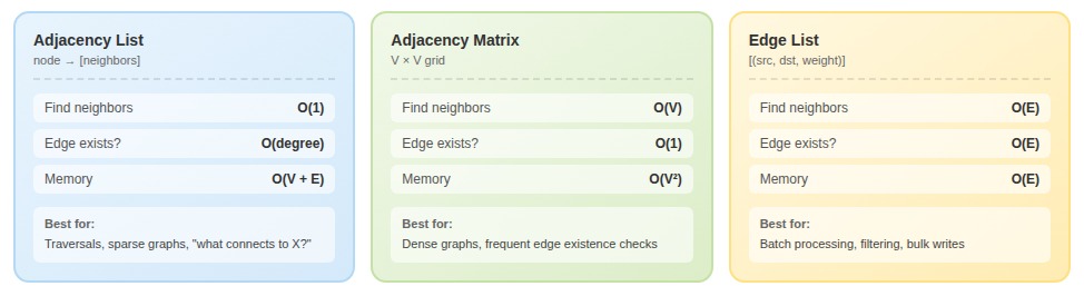
How to choose: What's your primary operation? "Find neighbors and traverse" means adjacency lists. Thousands of edge existence checks per second means matrices for dense graphs or adjacency lists with neighbor sets for sparse graphs. Bulk transformations make edge lists underrated.

Production systems rarely have a single workload. What actually works is often hybrid: store an adjacency list for traversals, maintain a hash set of edges for O(1) existence checks. Memory cost doubles, but you've eliminated the bottleneck.

Graph performance at scale: supernodes and indexes

In most real-world graphs, degree distribution follows a power law: a small number of nodes have vastly more connections than average. Twitter has users with 100 million followers. Amazon has products with millions of reviews.

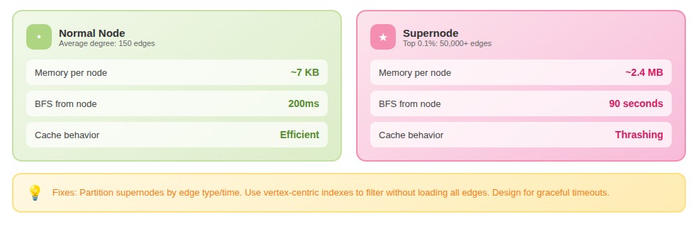
These supernodes break assumptions baked into standard algorithms. Traversing from a supernode means touching millions of edges. Storing its adjacency list consumes disproportionate memory. Query performance becomes bimodal: fast for normal nodes, catastrophically slow when a supernode appears in the path.

One team's graph analytics worked perfectly in development; their test graph capped node degree at 10,000. In production, they hit a supernode with 2.3 million edges. A single BFS consumed 40GB of memory and took 90 seconds.

The solutions aren't pretty but they work: 

• Partition supernodes by edge type or time window (splitting one node into many)
• Use vertex-centric indexes to filter edges without loading all of them
• Accept that some queries will be slow and designed for graceful timeouts

Indexes dominate real-world performance. A team ran multi-hop queries across a product knowledge graph with 8M nodes and 40M edges. Naive traversal: 45 seconds. After adding targeted indexes on edge types, compatibility attributes, and reverse edges, query time dropped to 1.2 seconds. Storage increased 30%. Same algorithm, same graph structure, the difference was avoiding linear scans at every traversal step.

Why graph structures matter for AI training

We've seen the shift in what labs request. 

Three years ago, most training data contracts were text: documents, conversations, code. Now roughly 40% of our advanced projects involve relationship annotation: entity graphs, dependency structures, knowledge bases. The models need to learn patterns that flat text doesn't teach.

Give a model Wikipedia articles mentioning Paris, the Eiffel Tower, and Gustave Eiffel, and it learns associations. 

Give it a knowledge graph with typed edges (Paris -[contains]-> Eiffel Tower, Gustave Eiffel -[designed]-> Eiffel Tower) and it learns something qualitatively different. It learns relationship patterns that transfer.

There's something philosophically interesting here: a graph forces you to make relationships explicit. In text, the connection between Gustave Eiffel and his tower is implied: you infer it from context, from proximity, from world knowledge. 

In a graph, you have to name it. "Designed." That naming act is a form of understanding. When annotators create these edges, they're not just labeling data. They're encoding judgments about what relationships are salient enough to matter. The model learns from those judgments. The annotator's understanding of what matters becomes the model's understanding of what matters.

Quality beats quantity for relationship-heavy data 

A research team building training data for code understanding had two options: 50,000 repository dependency graphs extracted automatically (with a roughly 15% error rate), or 2,000 dependency graphs manually verified by annotators. The annotators weren't general contractors; they were developers with production experience who understood why a package might depend on another. 

Synthetic generation hits fundamental limits 

We've seen synthetic generation hit a wall for graph-structured data. The problem is that graphs have global consistency requirements that local generation processes struggle to maintain. A model fine-tuned to output entity triples produces locally plausible results, but when composed into a graph, you get contradictions. 

One lab tried synthetic graph generation for six months before switching to human annotation. Their conclusion: synthetic works for augmentation (varying existing structure) but not for creating novel high-quality graph data from scratch. This matches what we see across domains. 

Synthetic generation can produce infinite variations. Only humans know which variations matter. A graph isn't just a structure; it's a structure that means something. The "designed" edge between Gustave Eiffel and the Eiffel Tower encodes a judgment about what relationship is salient. Synthetic processes optimize for plausibility. Human annotation optimizes for meaning.

Contribute to AI training at DataAnnotation

The graph structures powering recommendation engines, knowledge graphs, and relationship modeling in frontier AI require training data that captures genuine patterns, not synthetic shortcuts.

When you're teaching models to understand relationships, hierarchies, and network effects, quality of examples matters more than quantity. That work requires people who understand not just what graphs represent, but why certain structures matter and how relationships encode meaning.

Over 100,000 remote workers contribute to this infrastructure. Getting started takes five steps:

1. Visit the DataAnnotation application page and click "Apply"
2. Fill out the brief form with your background and availability
3. Complete the Starter Assessment—it tests critical thinking, not checkbox compliance
4. Check your inbox for the approval decision (typically within a few days)
5. Log in to your dashboard, choose your first project, and start earning

No signup fees. DataAnnotation stays selective to maintain quality standards. The Starter Assessment can only be taken once, so read instructions carefully before submitting.

Apply to DataAnnotation if you understand why graph quality requires human expertise and have the domain knowledge to contribute.