Types of Graphs: Why Classification Determines Which Algorithms Work

Your pathfinding algorithm returns nonsense. The code is correct. The logic is sound. The graph has weights, and you ran BFS.

That single mismatch (weighted graph, unweighted algorithm) is why graph classification matters. It determines which algorithms work, which optimizations apply, and which operations are even possible. Run cycle detection on a DAG, and you waste compute on a structural guarantee you already had. Treat a directed graph as undirected, and your results are wrong in ways that won't throw errors.

Graph types are not taxonomic trivia. They are constraints that determine what you can compute efficiently, what you can compute at all, and what you waste resources attempting when the structure already gives you the answer.

Graph classification: the core dimensions

Graph properties are independent dimensions that combine. A graph can be directed AND weighted AND cyclic AND disconnected. Each property enables or disables specific algorithm families.

Understanding these dimensions prevents the most common graph algorithm failures in production systems.

Directed vs. undirected graphs

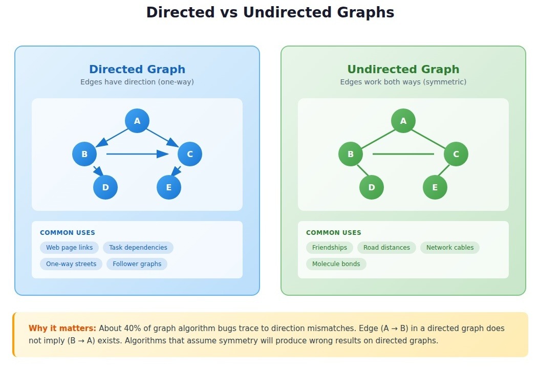
Direction changes everything about which algorithms apply and what results mean.

• Directed graphs represent relationships with inherent asymmetry: web pages linking to each other, task dependencies, one-way streets, follower relationships. Edge (A → B) exists independently of edge (B → A).
• Undirected graphs represent symmetric relationships: friendships, physical distances, electrical connections. Edge (A — B) implies traversal works both directions.

A machine learning engineer building recommendation systems at an e-commerce company implemented collaborative filtering on what she assumed was an undirected "users who bought similar products" graph. The algorithm kept producing bizarre recommendations.

The graph was actually directed. User A buying products similar to User B does not mean B's purchasing pattern should influence A's recommendations with equal weight. The asymmetry was semantic, not structural, and the algorithm could not learn it.

About 40% of graph algorithm bugs we debug in production code trace back to direction mismatches: treating directed graphs as undirected or misapplying directed algorithms to undirected structures.

Common directed graph algorithms:

• Topological sort (DAGs only)
• Strongly connected components (Tarjan's, Kosaraju's)
• PageRank and other centrality measures

Common undirected graph algorithms:

• Connected components (BFS/DFS)
• Minimum spanning tree (Prim's, Kruskal's)
• Bridge and articulation point detection

Weighted vs. unweighted graphs

Edge weights are not decoration. They are operational data that determines whether your algorithm produces meaningful results or confident garbage.

• Unweighted graphs treat all edges as equivalent. The "distance" between connected nodes is always 1. Social networks (friend or not friend), dependency graphs (depends or does not depend), and reachability problems often use unweighted representations.
• Weighted graphs assign numerical values to edges representing cost, distance, capacity, or probability. Road networks, network latency, financial transactions, and similarity scores require weights.

The most common failure mode: engineers implement BFS for shortest path problems when their graph has weights. BFS finds the path with fewest edges, not the path with lowest total weight.

A mapping application returned absurd routes. Technically the fewest turns, the algorithm routed through slow residential streets instead of highways. Someone had used BFS on a weighted road network.

Algorithm selection by weight:

On a graph with 100,000 nodes, BFS completes in milliseconds while Dijkstra's takes several seconds. But if your graph has weights and you run BFS, those milliseconds produce wrong answers.

Cyclic vs. Acyclic Graphs

Whether your graph contains cycles determines which entire algorithm categories apply.

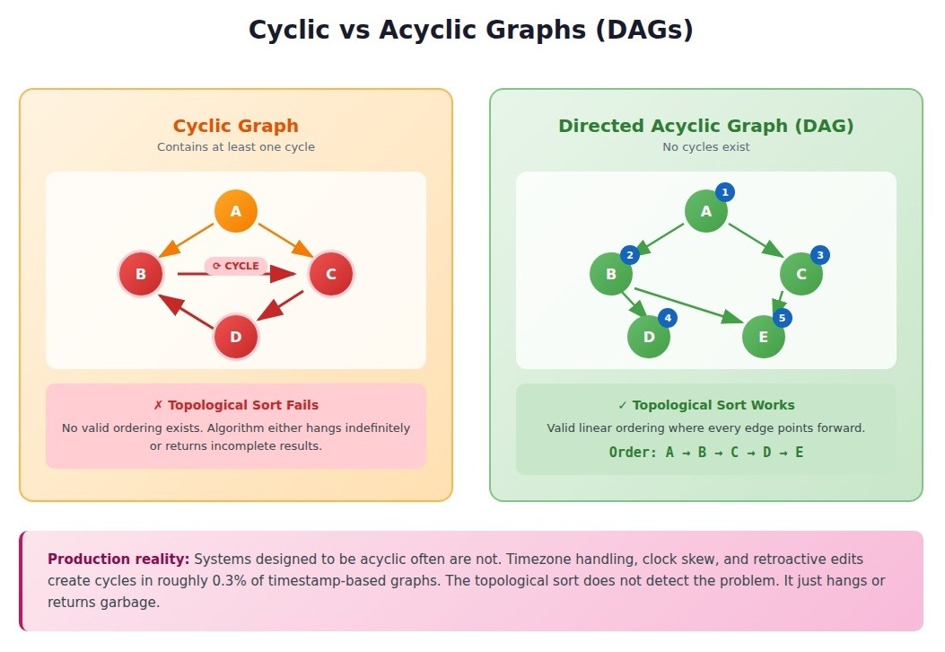
• Cyclic graphs contain at least one path that returns to its starting node. Social networks, road networks, and most real-world graphs are cyclic.
• Acyclic graphs contain no cycles. Directed acyclic graphs (DAGs) are particularly important: dependency trees, version histories, neural network architectures, and scheduling problems.

DAGs unlock algorithms that fail catastrophically on cyclic graphs. Topological sorting produces a linear ordering where every edge points forward. It only works on DAGs. Run it on a cyclic graph, and it either hangs forever or returns incomplete results.

A monorepo build system with 3,000 packages and 12,000 dependency edges would hang indefinitely when developers accidentally created circular dependencies. The topological sort was not designed to detect cycles. It just looped. The longest hang we traced lasted 47 minutes before someone killed the process.

A senior build engineer who maintained the system for four years could find cycles in under a minute with the right visualization. Always the same pattern: a dev dependency that should be a peer dependency. That recognition came from years of incidents. The algorithm could not learn it.

Why cycles hide in "acyclic" data

Systems designed to be acyclic often are not. Timestamp-based graphs where edges point from older to newer nodes should guarantee acyclic structure by construction. In document processing systems, we found that timezone handling, clock skew, and retroactive editing create cycles in roughly 0.3% of cases. Negligible until you process millions of documents.

The cycle detection trade-off

Standard cycle detection using depth-first search is O(V + E), linear in graph size. Efficient in theory. In a high-throughput system running detection on every graph ingestion, it reduced throughput by 35%.

The optimal approach depends on cycle frequency:

class CycleDetectedError(Exception):
    pass


def topological_sort_optimistic(graph):
    """Assume acyclic, detect cycle only on failure. 
    Optimal when cycles are rare (<5% of graphs)."""
    in_degree = {node: 0 for node in graph}
    for node in graph:
        for neighbor in graph[node]:
            in_degree[neighbor] = in_degree.get(neighbor, 0) + 1

    queue = [node for node, degree in in_degree.items() if degree == 0]
    result = []

    while queue:
        node = queue.pop(0)
        result.append(node)
        for neighbor in graph[node]:
            in_degree[neighbor] -= 1
            if in_degree[neighbor] == 0:
                queue.append(neighbor)

    if len(result) != len(in_degree):
        raise CycleDetectedError("Graph contains cycle")
    return result


def has_cycle(graph):
    """O(V+E) cycle detection. Run upfront when cycles are common (>5%)."""
    WHITE, GRAY, BLACK = 0, 1, 2
    color = {node: WHITE for node in graph}

    def dfs(node):
        color[node] = GRAY
        for neighbor in graph.get(node, []):
            if color[neighbor] == GRAY:
                return True
            if color[neighbor] == WHITE and dfs(neighbor):
                return True
        color[node] = BLACK
        return False

    return any(dfs(node) for node in graph if color[node] == WHITE)

Cycles were rare enough in the build system (about 2%) that paying detection cost upfront penalized 98% of cases. The optimistic approach worked: assume acyclic, catch the exception when topological sort fails, run detection only on failures.

Connected vs. disconnected graphs

A graph's connectivity determines which algorithms produce meaningful results.

• Connected graphs have a path between every pair of nodes (undirected) or every pair is reachable in at least one direction (weakly connected for directed graphs).
• Disconnected graphs contain multiple components with no edges between them. Many real-world graphs are disconnected: user networks with isolated communities, document collections with unrelated topics, infrastructure with air-gapped segments.

A social network analysis tool reported bizarre clustering results. The community detection algorithm assumed the graph was connected. The actual graph had thousands of disconnected components. The algorithm tried to optimize a global metric across components with no relationship, producing meaningless partition boundaries.

def find_connected_components(graph):
    """Run BEFORE algorithms that assume connectivity."""
    visited = set()
    components = []

    def bfs(start):
        component = []
        queue = [start]
        while queue:
            node = queue.pop(0)
            if node in visited:
                continue
            visited.add(node)
            component.append(node)
            queue.extend(graph.get(node, []))
        return component

    for node in graph:
        if node not in visited:
            components.append(bfs(node))

    return components


# Always check before running global algorithms
components = find_connected_components(graph)
if len(components) > 1:
    print(f"Warning: {len(components)} disconnected components")
    # Run algorithm per component, not globally

The fix is straightforward: run component detection first. Most teams do not know to check.

Bipartite graphs

A bipartite graph has nodes divisible into two disjoint sets where every edge connects a node from one set to a node in the other. No edges exist within sets.

Common examples: job applicants and positions, users and products, students and courses, documents and terms.

Bipartite structure enables specialized matching algorithms (Hungarian algorithm, Hopcroft-Karp) that do not apply to general graphs. Attempting to run bipartite matching on a non-bipartite graph produces undefined behavior.

Bipartiteness test: A graph is bipartite if and only if it contains no odd-length cycles. BFS-based two-coloring detects this in O(V + E).

def is_bipartite(graph):
    """Returns (True, partition) if bipartite, (False, None) otherwise."""
    color = {}
    
    for start in graph:
        if start in color:
            continue
        queue = [start]
        color[start] = 0
        
        while queue:
            node = queue.pop(0)
            for neighbor in graph.get(node, []):
                if neighbor not in color:
                    color[neighbor] = 1 - color[node]
                    queue.append(neighbor)
                elif color[neighbor] == color[node]:
                    return False, None
    
    set_a = {n for n, c in color.items() if c == 0}
    set_b = {n for n, c in color.items() if c == 1}
    return True, (set_a, set_b)

Trees: the constrained graph

A tree is a connected acyclic undirected graph. Every tree with N nodes has exactly N-1 edges. Adding any edge creates a cycle. Removing any edge disconnects the graph.

Trees are graphs with maximum constraint: connected (one component), acyclic (no cycles), and minimally connected (fewest possible edges). These constraints enable efficient algorithms:

• Unique paths: Exactly one path exists between any two nodes
• O(N) traversal: BFS and DFS visit every node exactly once
• Root-based algorithms: Choosing a root enables parent-child relationships

Binary search trees, decision trees, file system hierarchies, and DOM structures are all trees. Recognizing tree structure unlocks simpler algorithms than general graph approaches require.

Special graph types

• Multigraphs: Allow multiple edges between the same pair of nodes. Represent parallel routes, multiple relationships, or repeated interactions. Many graph libraries do not support multigraphs natively.
• Hypergraphs: Edges connect arbitrary numbers of nodes, not just pairs. Represent group relationships: co-authorship, chemical reactions, set membership. Require specialized representations.
• Planar graphs: Can be drawn on a plane with no edge crossings. Enable specialized algorithms for maps, circuit layouts, and geographic problems.

Algorithm selection: the decision framework

Graph properties combine to determine which algorithms apply. Use this framework:

Shortest path selection

1. Is the graph weighted?
   
   • No → BFS (O(V + E))
   • Yes → Continue
2. Are any weights negative?
   
   • No → Dijkstra's (O((V + E) log V))
   • Yes → Continue
3. Could negative cycles exist?
   
   • No → Bellman-Ford (O(V × E))
   • Yes → No solution; detect and report

Traversal selection

1. Need level-by-level processing? → BFS
2. Need to explore deeply before backtracking? → DFS
3. Need linear ordering of DAG? → Topological sort
4. Need to process nodes by priority? → Priority queue (Dijkstra's pattern)

Connectivity selection

1. Undirected graph components? → BFS/DFS component detection
2. Directed graph strong components? → Tarjan's or Kosaraju's algorithm
3. Need to find bridges/articulation points? → Specialized DFS variants

What tutorials get wrong about graph classification

Most tutorials present graph properties as things you know about your data. They are actually things you discover.

The tutorials say: "If your graph is acyclic, use topological sort."

But you do not know if your graph is acyclic. You have a belief, based on how you designed the system, that it should be acyclic. The graph's actual structure is ground truth. Your beliefs about it are hypotheses.

This matters because:

1. Data evolves. A graph that was acyclic during development gains cycles in production through edge cases, user behavior, or integration with external systems.
2. Assumptions compound. If Algorithm A assumes acyclicity and Algorithm B assumes connectivity, running both requires both properties to hold simultaneously.
3. Silent failures are expensive. Wrong algorithm choices often produce wrong results without errors. The mapping application with BFS on weighted graphs did not crash. It returned bad routes that users complained about for weeks before anyone traced the cause.

The production-grade approach: verify properties before depending on them, or design systems to detect and handle violations gracefully.

Graph properties as data quality signals

In AI training contexts, graph structure reveals data quality issues that surface-level inspection misses.

Entity resolution example: A team building training datasets for entity extraction represented "same as" relationships as edges. Connected component analysis should produce one component per real-world entity.

The product entity graph had 47 connected components for variations of "iPhone." The resolution rules were not wrong. Annotators were making different judgment calls about what counted as "the same product."

A consumer electronics specialist resolved it in an afternoon. The iPhone 14 Pro and iPhone 14 Pro Max have different SKUs but the same product line. Annotators without retail experience could not know that distinction matters. The component count dropped from 47 to 3.

That judgment was not in the data. It was domain expertise that graph structure revealed was missing.

Apply graph expertise to AI development

The graph structures shaping modern AI systems (knowledge graphs, neural architectures, dependency networks) all rely on classification decisions that determine performance characteristics.

Understanding which properties enable which optimizations, recognizing that structural assumptions break algorithms silently, knowing when to verify versus when to assume: that judgment comes from technical depth, not surface-level definitions.

Frontier models processing these structures at scale need training data created by people who think in terms of constraints, properties, and algorithmic implications.

If your background includes technical expertise, domain knowledge, or the critical thinking to evaluate complex trade-offs, DataAnnotation positions that expertise at the frontier of AGI development.

To join over 100,000 contributors building this infrastructure:

1. Apply at DataAnnotation
2. Complete the Starter Assessment (one attempt; read instructions carefully)
3. Receive approval (typically within days)
4. Select projects matching your expertise and start contributing

No fees. Flexible hours. Compensation reflects the technical depth required.