Top-P Sampling: What Is It and Why Does It Matter?

Two teams evaluated the same production model last month. Same architecture, same training data, same prompts. One team reported 89% task accuracy. The other measured 72%.

The difference wasn't the model; it was the top-p setting: 0.9 vs. 0.95.

That 0.05 difference changed how the model selected every token. Same architecture. Same weights. But generation behavior shifted enough that one team nearly rejected a model the other team shipped to production.

This is the kind of evaluation noise the industry mistakes for signal. Sampling parameters like top-p don't just affect output quality; they change how your model appears to perform.

What is top-p sampling?

Top-p sampling is a text generation method in which the model samples only from tokens whose cumulative probability exceeds a threshold p. Unlike top-k sampling, which always considers exactly k tokens, top-p adapts the candidate pool to the model's confidence, keeping few tokens when confident and many when uncertain.

When I audit model deployments that underperform expectations, sampling parameters rank just behind prompt construction as the culprit. Engineers tune their prompts extensively, run evaluation sets, and obtain stakeholder sign-off. Then someone changes top-p from the default, and output quality shifts in ways that don't show up until production.

How does top-p sampling work? 

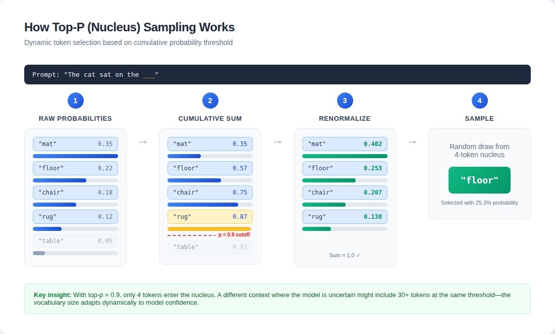
Here's the mechanism: the model produces a probability distribution over its entire vocabulary (typically 50,000+ tokens). For a completion like "The cat sat on the ___", you might see:

# Token probability distribution for "The cat sat on the ___"
probs = {
    "mat": 0.35,
    "floor": 0.22,
    "chair": 0.18,
    "rug": 0.12,
    "table": 0.05,
    "banana": 0.0003,
    # ... tens of thousands more tokens
}

The algorithm sorts these probabilities in descending order, then accumulates them until reaching your top-p threshold. With top-p at 0.9, it walks down the sorted list until crossing 0.9 cumulative probability. Everything below that cutoff is completely zeroed out, then remaining probabilities get renormalized to sum to 1.0 before sampling.

def nucleus_sample(probs: dict, top_p: float = 0.9):
    # Sort tokens by probability (descending)
    sorted_tokens = sorted(probs.items(), key=lambda x: x[1], reverse=True)

    # Accumulate until reaching top_p threshold
    cumulative = 0.0
    nucleus = {}
    for token, prob in sorted_tokens:
        cumulative += prob
        nucleus[token] = prob
        if cumulative >= top_p:
            break

    # Renormalize to sum to 1.0
    total = sum(nucleus.values())
    return {t: p / total for t, p in nucleus.items()}

The critical property is dynamic vocabulary size. On one token, if the model is highly confident, top-p of 0.9 might keep only 2–3 candidates. If uncertain, the same parameter might preserve 50+ options. This creates output patterns that look inconsistent until you realize the model's confidence varies dramatically across different parts of the same response.

The original researchers used "nucleus" as a metaphor: keep the dense core of the probability distribution and discard the long tail. But the metaphor misleads. The "nucleus" isn't semantically coherent; it's statistically coherent. When generating technical content, top-p at 0.9 might keep six plausible-sounding terms, three of which are technically incorrect for the context. The probability distribution reflects training data, not ground truth.

Top-p changes can mask or reveal model weaknesses. Set it high (0.95–1.0), and models sample from long tails of low-probability tokens, exposing training gaps through occasional nonsensical outputs. Set it low (0.7–0.85), and models stick to high-confidence predictions, hiding uncertainty but sometimes producing repetitive text when no single continuation has strong probability mass.

How sampling parameters interact

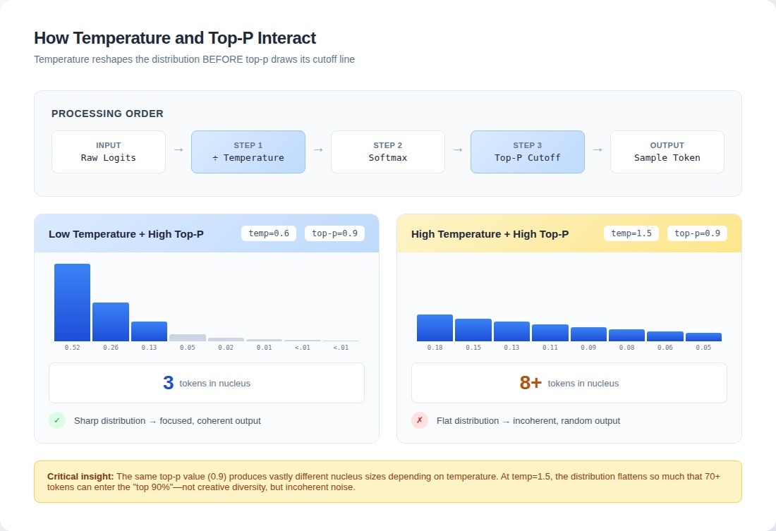
Top-p doesn't operate in isolation. Temperature gets applied first, reshaping the distribution that the nucleus then cuts. Temperature divides logits and changes their relative spread; softmax converts them to probabilities; only then does top-p draw its cutoff line.

import numpy as np

def generate_with_sampling(
    logits: np.ndarray, 
    temperature: float = 1.0, 
    top_p: float = 0.9
):
    """
    Generates samples from logits using temperature scaling and top-p (nucleus) sampling.

    Args:
        logits (np.ndarray): Raw model outputs (before softmax).
        temperature (float): Controls randomness; higher -> more random.
        top_p (float): Cumulative probability threshold for nucleus sampling.

    Returns:
        tuple: (selected_indices, probabilities of selected indices)
    """

    # Step 1: Apply temperature scaling (before softmax)
    scaled_logits = logits / temperature

    # Step 2: Convert logits to probabilities using softmax
    exp_logits = np.exp(scaled_logits - np.max(scaled_logits))  # subtract max for stability
    probs = exp_logits / exp_logits.sum()

    # Step 3: Perform top-p (nucleus) filtering
    sorted_indices = np.argsort(probs)[::-1]        # Sort probabilities descending
    cumulative = np.cumsum(probs[sorted_indices])  # Cumulative sum
    cutoff_idx = np.searchsorted(cumulative, top_p) + 1  # Find cutoff for top-p

    nucleus_indices = sorted_indices[:cutoff_idx]         # Keep top-p indices
    return nucleus_indices, probs[nucleus_indices]

The parameters don't combine linearly. At temperature 0.3 with top-p 0.95, you get one behavior. Bump temperature to 1.2 while keeping top-p at 0.95, and output quality can collapse entirely for certain task types.

A model configured with temperature 1.5 and top-p 0.9 flattened the distribution so much that the top-90% nucleus included seventy tokens instead of fifteen. The model didn't produce diverse creative output—it produced incoherent garbage. Dropping temperature from 1.0 to 0.6 can cut the effective nucleus from 40 tokens to 8 at the same top-p value.

Top-k and min-p represent alternative or complementary filtering strategies. When you combine top-k with top-p, top-k acts first: it reduces the candidate set to exactly k tokens, then top-p considers only those. This can create situations where top-p becomes a no-op. If your top-k is set to 20 and your top-p would naturally include 40 tokens, the top-k constraint binds. Min-p provides a floor that top-p alone can't guarantee, preventing truly low-probability tokens from entering the nucleus during high-temperature generation.

How sampling parameters affect evaluation

Most public benchmarks report scores without specifying sampling parameters, or they use greedy decoding by default. This isn't an oversight, it's a systematic blind spot that makes leaderboard rankings essentially meaningless for production decisions.

A model that tops the leaderboard with greedy decoding might perform worse with nucleus sampling enabled. Another model might show the opposite pattern. If your benchmark only tests one configuration, you're measuring a model's fit to a specific decoding strategy, not its general capability. This matters when comparing LLMs for specific tasks; the "best" model depends heavily on how you configure generation.

Greedy decoding is deterministic; run the same prompt twice, get identical output. But high accuracy scores with greedy decoding don't mean production-ready. Testing on question-answering tasks showed this pattern: a model evaluated with greedy decoding achieved 89% accuracy. With top-p 0.9 and temperature 0.8, running the same questions five times each, per-question accuracy dropped to 84%. But scoring the best-of-five answers pushed accuracy to 93%. The model had learned distributions that greedy decoding was exploiting poorly.

The solution isn't abandoning benchmarks. It's controlling sampling parameters as explicitly as other evaluation variables. At minimum, test across greedy decoding (temperature 0), moderate sampling (top-p 0.9, temperature 0.7), and high-diversity sampling (top-p 0.95, temperature 1.0). For each configuration, multiple samples per test case quantify variance.

Choosing a decoding strategy

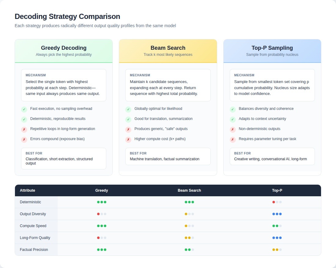
No decoding strategy wins universally. The same model produces radically different output quality profiles depending on whether it uses top-p, beam search, or greedy decoding.

Beam search optimizes for the most likely sequence according to the model's probability distribution. In practice, "most likely" often means "most generic." A creative writing assistant built with beam search generated technically coherent story continuations, but users complained output felt repetitive and predictable. Switching to top-p at 0.9 improved output quality: the model began taking narrative risks, introducing unexpected plot elements that users loved. But evaluation metrics initially worsened because outputs diverged further from reference continuations.

The opposite problem happens too. A legal document analysis system switched from beam search to top-p because someone read that top-p produces "more natural" outputs. Accuracy on contract clause extraction dropped 12%.

Greedy decoding always selects the single highest-probability token. For certain tasks, it outperforms sophisticated approaches while running significantly faster. Testing greedy versus top-p on a classification task wrapped in a generative interface: greedy achieved 94% accuracy, top-p at 0.9 achieved 91%. The randomness added nothing but noise. One team saved $4,000 monthly in GPU costs by switching from top-p to greedy for their intent classification endpoint.

But greedy fails catastrophically at longer-form generation due to exposure bias. During training, models see ground-truth context. During greedy decoding, they see their previous outputs, and small errors compound. Text that starts coherently can degrade into repetitive loops after 200 tokens. Top-p sampling introduces enough randomness to break these failure patterns. The context window compounds this problem; as generation extends, the model attends to its own potentially degraded output rather than high-quality training examples.

Task-specific patterns from operational data:

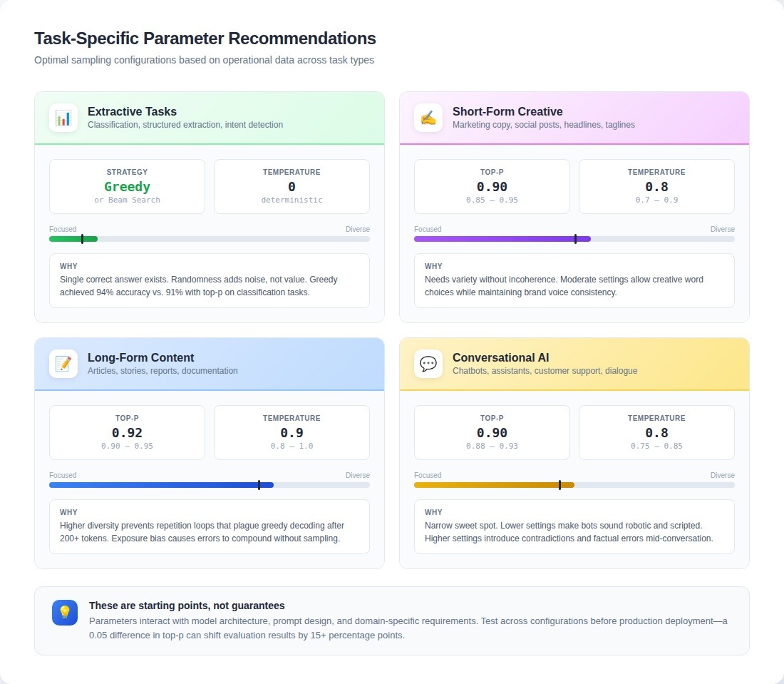
• Extractive tasks (classification, structured data extraction): Greedy decoding or beam search consistently outperforms sampling methods
• Short-form creative generation: Top-p 0.85–0.95 with temperature 0.7–0.9 produces the best balance
• Long-form content generation: Top-p 0.9–0.95 with temperature 0.8–1.0 prevents repetition loops
• Conversational AI: Top-p 0.88–0.93 with temperature 0.75–0.85 hits the sweet spot. Lower settings make bots sound scripted; higher settings introduce contradictions

Why this matters for AGI development

These aren't implementation details. The systems evaluating frontier models face the same sampling parameter problem at unprecedented scale.

When human evaluators rate model outputs, they're rating the interaction between model capabilities and generation settings, often without knowing which settings produced what they're seeing. A model that looks brilliant with top-p at 0.85 might look incoherent at 0.98. The evaluator rates what they see. The rating becomes training signal. The model learns from feedback that was really about sampling strategy, not about what makes outputs genuinely good.

That gap between what automated metrics measure and what actually matters, that's where human judgment creates value.

Contribute to AGI development at DataAnnotation

To understand whether top-p at 0.9 produces better results than 0.95, you must compare thousands of generations across diverse prompts, rate quality systematically, and identify patterns that distinguish coherent creativity from random noise.

That evaluation depends on human judgment that understands the difference between technically valid outputs and genuinely useful ones. As generation strategies grow more sophisticated, the competitive advantage shifts to organizations whose evaluation infrastructure can measure what actually matters.

If your background includes technical expertise, domain knowledge, or the critical thinking to evaluate complex trade-offs, AI training at DataAnnotation positions you at the frontier of AGI development. Over 100,000 remote workers have contributed to this infrastructure.

1. Visit the DataAnnotation application page and click "Apply"
2. Fill out the brief form with your background and availability
3. Complete the Starter Assessment, which tests your critical thinking skills
4. Check your inbox for the approval decision (typically within a few days)
5. Log in to your dashboard, choose your first project, and start earning

No signup fees. DataAnnotation stays selective to maintain quality standards. You can only take the Starter Assessment once, so read the instructions carefully and review before submitting. Apply to DataAnnotation.